Carol Johnston
TWI Ltd, Granta Park Great Abington, Cambridge, CB21 6AL, UK
Paper presented at the ASME 2017 36th International Conference on Ocean, Offshore and Arctic Engineering, OMAE2017, June 25-30, 2017, Trondheim, Norway
Abstract
The offshore environment contains many sources of cyclic loading. Standard design S-N curves, such as those in DNVGL-RP-C203, are usually assigned to ensure a particular design life can be achieved for a particular set of anticipated loading conditions. Girth welds are often the ‘weak link’ in terms of fatigue strength and so it is important to show that girth welds made using new procedures for new projects that are intended to be used in fatigue sensitive risers or flowlines do indeed have the required fatigue performance. Alternatively, designers of new subsea connectors, used for example in tendons for tension leg platforms, mooring applications or well-heads which will experience cyclic loading in service, also wish to verify the fatigue performance of their new designs. Often operators require contractors to carry out resonance fatigue tests on representative girth welds in order to show that girth welds made using new procedures qualify to the required design S-N curve. Operators and contractors must then interpret the results, which is not necessarily straightforward if the fatigue lives are lower than expected.
Many factors influence a component’s fatigue strength so there is usually scatter in results obtained when a number of fatigue tests are carried out on real, production standard components. This scatter means that it is important first to carry out the right number of tests in order to obtain a reasonable understanding of the component’s fatigue strength, and then to interpret the fatigue test results properly. A working knowledge of statistics is necessary for both specifying the test programme and interpreting the test results and there is often confusion over various aspects of test specification and interpretation.
This paper describes relevant statistical concepts in a way that is accessible to non-experts and that can be used, practically, by designers. The paper illustrates the statistical analysis of test data with examples of the ‘target life’ approach (that is now included in BS7608:2014 + A1) and the equivalent approach in DNVGL-RP-C203, which uses the stress modification factor. It gives practical examples to designers of a pragmatic method that can be used when specifying test programmes and interpreting the results obtained from tests carried out during qualification programmes, which for example, aim to determine whether girth welds made using a new procedure qualify to a particular design curve. It will help designers who are tasked with specifying test programmes to choose a reasonable number of test specimens and stress ranges, and to understand the outcome when results have been obtained.
1. Introduction
A common approach for quantifying fatigue life is using SN curves, which plot stress versus endurance. In standards such as BS7608 [1] and DNVGL-RP-C203 [2], welds are grouped based on the direction of applied stress with respect to the weld and the weld geometry. A fatigue “Class” therefore provides designers with information about a specific weld’s resistance to fatigue stresses.
The fatigue classes that are now contained within BS7608 were originally obtained by statistical analysis of large datasets of test results. In addition to gathering test data from the literature, specific test programmes were carried out on relevant weld details, such as welded attachments, in order to generate appropriate data. Test results from details which had similar fatigue strength were grouped together and a combination of statistical analysis and engineering judgement was used to define nine fatigue classes [3]. The first set of design rules, BS5400 was published in 1980 [4] and contained the mean and design curves for various fatigue classes that had (mainly) been obtained by regression analysis. Since statistical analysis of datasets was used to obtain the fatigue Classes within, BS7608 each Class has its own specific standard deviation of Log N associated with it. The fatigue section of the DNV rules [5] was based on the same nine classes. However, rather than giving individual Classes different standard deviations, the approach in DNV-RP-C203 was to apply a single value of standard deviation to all of the classes. This is equal to 0.2 for the main classes.
Given that many factors affect fatigue strength, it is advisable to carry out tests in order to confirm the fatigue strength of new components or of girth welds made with new welding procedures. It is often a requirement by operators for contractors to carry out fatigue tests on representative girth welds in order to confirm that the girth welds made using new procedures do qualify to the required design S-N curve and so have sufficient fatigue strength.
Fatigue test programmes for welds involve choosing a sample, choosing relevant test parameters, analysing the results and making a judgement about whether the welds tested do indeed have the required fatigue endurance. Choosing the number of samples to test and analyzing the results both require knowledge of statistics and there can be some confusion over aspects of test specification and interpretation of test results. This paper aims to explain the process of specifying the test programme and interpreting the test results for those who are not experts in statistics. For simplicity, the example used throughout will be the qualification of girth welds via full scale resonance fatigue testing.
2. Relevant concepts
Endurance - N, is the number of applied cycles. An SN curve plots Log N on the x-axis (Figure 1).
Stress range - S, is the parameter describing the cyclic stress, in which the applied stress varies with time from a maximum to a minimum value. When considering the fatigue endurance of welds, the full stress range ie maximum stress minus minimum stress (as opposed to the stress amplitude) is relevant. An SN curve plots Log S on the y-axis (Figure 1).
Normal distribution - Statistical concept which predicates the probability that a particular value of a continuous, large dataset will occur. It is symmetrical about the mean value, and its width is quantified by its standard deviation.
Scatter - Many factors influence fatigue strength and so a range of fatigue lives is often obtained for tests carried out at the same stress range on nominally identical, production-standard components, ie there is ‘scatter’ in results. In large datasets of fatigue test results with lives below around 2 million cycles, the logarithm of the endurances (Log N) follow a normal distribution [3]. By definition of a two-sided prediction interval for a normal distribution, 95% of the data lies within 1.96 standard deviations of the mean. However, when considering fatigue design, the designer is usually only concerned with showing that the component being considered will have a life that is longer than a particular value, and so fatigue design is concerned with one-sided prediction limits instead (Figure 2). For one-sided prediction limits, 1.96 standard deviations corresponds to 95.5% of the results, whereas 2 standard deviations corresponds to 97.7%. By definition, fatigue design curves are located 2 standard deviations below the mean, which means that 97.7% of the results lie above the design curve.
Figure 1 - An SN curve showing a representation of scatter in fatigue test data
Figure 2 - The difference between two-sided and one-sided prediction limits for a normal distribution
Standard deviation - SD, quantifies the scatter in a set of test results. The standard deviation relevant to SN curves quantifies the distribution of Log N about the mean SN curve. BS7608 provides different values of SD for each fatigue Class based on the statistical analysis that was carried out for each Class. In DNVGL-RP-C203, the standard deviation of all of the SN curves is assumed to equal 0.2.
SN curve - a plot of Log S (on the y-axis) versus Log N (on the x-axis). The mean SN curve is given by SmN = C. Using the equivalent logarithmic notation, this can be written as Log N = LogC - mLogS. For a large dataset, by definition, the design curve is two standard deviations below the mean curve. The design curve is therefore written as Log N = Log C -2SD -mLogS, where LogC is the intercept of the mean SN curve on the y axis and m is the slope. In certain standards (eg BS7608), both “mean” and “design” curves are provided. In others (eg DNVGL-RP-C203), only “design” curves are provided, in which case, Log N = Log CD -mLogS, where Log CD is the intercept of the design curve.
Sampling a population - A normally distributed variable (such as fatigue endurance of a large number of test results, like those used to derive the fatigue Classes), has a particular mean value (μ) and standard deviation (σ). When information on the fatigue strength of a new weld or component is required, it is impractical to carry out fatigue tests on a sufficient number of specimens to obtain the actual mean and standard deviation, therefore a sample of the population is taken by testing a small number of specimens. Since only a small number of specimens are tested, the mean (  ) and standard deviation (s) of the sample will be different from that of the whole population. The error in estimating μ by calculating is proportional to
  (termed the standard error on the mean, ) [6]. Note that the relevant standard deviation is that of the population not the sample. The standard deviation of the population is known when qualifying welds because the standard deviation from the standard SN curves can be used.
Dataset size - As noted above, it is customary to test a sample of a population. The inherent scatter in fatigue performance means that it is important to carry out an appropriate number of tests. There is often a balance to be struck between the number of tests that would give the result with highest level of statistical confidence and the cost implications of producing many full-scale test specimens.
Replication - in order to ensure that the fatigue tests carried out produce results which are representative of that weld, an appropriate number of repeat tests should be carried out at an appropriate number of stress ranges.
Student’s t distribution - statistical concept similar to the normal distribution which describes a continuous dataset of limited size. It is used when carrying out statistical tests on a small sample when the standard deviation of the population is unknown. Again, it is symmetrical about the mean and the width is again described in terms of its standard deviation, however to fully describe the function, the “number of degrees of freedom” must also be known, and this depends on the size of the dataset. Around 50 test results are needed for the Student’s t distribution to converge with the normal distribution.
Number of degrees of freedom ν - is defined as the number of test results minus the number of parameters to be estimated when analysing the results to obtain mean performance. It is a quantity used when calculating the Student’s t distribution. For example, if the Student’s t distribution is used during regression analysis of a fatigue test dataset of n results, and the aim is to determine both Log C and the slope, m, from the analysis, then ν = n - 2. If however m is forced to equal 3 (to match standard SN curves), then the analysis only needs to estimate Log C, and so ν = n - 1 [7].
Regression analysis - is used to derive the mean and the standard deviation of a dataset. When the dataset comprises test results (ie without any runouts, which would require a different statistical approach), regression analysis involves a least squares estimation of a line fitted to the test results, based on the observed values of the dependent variable about this line (Figure 3). The mean line is the one which minimizes the sum of squares of the residuals (di). Note that, for other applications, usually the dependent variable is plotted on the y-axis and so the residuals are between the mean and the y-values, however by convention, fatigue test data are plotted with the dependent variable (Log N) on the x-axis. As mentioned previously, when comparing fatigue test data to standard design curves, the slope is often fixed to match the design curve that the test results are being compared to.
Figure 3 - The concept of regression analysis of test results (blue points) as compared to the fitted mean line
The null hypothesis and the alternative hypothesis - these frame the question that is being answered when making a decision using statistical analysis. The “null hypothesis” for fatigue design is that the mean of the sample is equal to that of the population. There must also be an “alternative hypothesis” (and for fatigue design, it is that the mean of the sample is significantly greater than that of the population). Since the analysis is based on estimates of the population mean from the sample mean, there is a chance that the decision (and predictions based on it) will be incorrect (ie that the statistical test will say that the means are different when in fact they are not). The chance of this incorrect decision is quantified by the significance level [6].
Significance level, α - the significance level is a measure of the likelihood of incorrectly rejecting the null hypothesis based on the information obtained from a small sample (ie saying that the mean of the sample is greater than the population mean when in fact it is not). A significance level of 1% means such a prediction error is highly unlikely. A 5% significance means such a prediction error is moderately unlikely.
Confidence level - is another way to think of significance levels and is given by 1- α. When comparing means of a sample versus the population, the error in the predicted sample mean (-μ) is proportional to Using the concept of confidence levels, it is moderately unlikely that the error will be greater than  (where 1.645 is from standard normal distribution tables for a probability of 95%), and highly unlikely that it will be greater than
  (where 1.96 is the percentage point of a normal distribution for a probability of 97.5%). See BS600 [6] for further explanations. Ronald and Lotsberg [9] linked reliability with confidence levels and state that a 75% confidence is equivalent to a 10-4 failure probability for the last year of a 20-year design life.
Confidence limits give the limits within which a given population parameter (for example, the mean of the dataset) will lie.
3. Specifying a test programme
In practice, a sample size must be chosen when carrying out fatigue tests. In an ideal world, the fatigue strength of a component would be obtained by statistical analysis of test results from a large number of specimens. This would be impractical, costly and unrealistically time consuming for large-scale or full-scale tests. ASTM E379 [10] and BS ISO 12107 [11] both give advice on the number of specimens that should be tested.
ASTM E379-10 defines two types of tests:
- preliminary/exploratory tests or R&D testing of components.
- design allowables or reliability data
It discusses the replication level required when carrying out tests. It defines this as follows:
Replication, % = where Nσ is the number of stress levels used and n is the total number of tests.
For preliminary or R&D tests, it recommends that between 6 and 12 specimens should be tested. It states that a replication percentage of 17 to 33% is required for preliminary tests, whereas a replication percentage of 33 to 50% is needed for R&D testing. For “design allowables” or reliability data however, it recommends that 12 to 24 specimens should be tested, with a replication level of 50 to 75% to account for the higher degree of certainty required for this type of testing.
Using the SN approach, regression analysis is carried out on fatigue test data to produce a mean curve. ISO12107 provides guidance on statistical analysis and says that in order to “statistically verify the adequacy of a linear model, more than one specimen should be tested at each of three or more stress levels”. Using the definition of replication level above, this corresponds to a minimum requirement of a 50% replication rate on 6 tests ie testing two specimens at each of three stress levels.
Taking the two standards together, and looking at the minimum numbers of specimens recommended in each, for preliminary tests the minimum number of specimens in a test programme for ISO12107 (6) with the minimum ASTM replication level (17%) would not be appropriate because this corresponds to a programme involving four stress ranges with only two repeat tests. This does not conform to the requirements of ISO12107. Instead, if six specimens are tested, a replication rate of 50% is required (ie two tested at each of three stress ranges) to satisfy ISO12107, and this corresponds to the highest required replication rate for R&D tests in ASTM379-10.
In order to satisfy both standards when obtaining design data through testing and gain a reliable understanding of fatigue strength, ASTM requires a minimum of 12 specimens to be tested. The replication level which results in the fewest number of stress levels is 75% This corresponds to four tests at each of three stress levels. This also satisfies ISO12107, which states that at least two tests at each of three stress levels. This is summarized in Table 1.
It has become standard industry practice for Operators and Contractors to require two or three tests to be carried out at each of three stress ranges when specifying girth weld qualification test programmes. Depending on the purpose of the test programme, it should be noted that this does not necessarily comply with recommendations in these two standards. As noted above, a test programme to produce design data would comprise a minimum of 12 specimens, with four being tested at each of three stress ranges. The most pragmatic approach for resonance fatigue tests on girth welded pipes would be have six pipes each containing two welds and test two pipes (ie four welds) at each of three stress ranges. In this situation at a minimum, two results would be obtained at each of three stress ranges. The second weld in each pipe would be a runout and so have a life at least as long as that of the cracked weld, and this is enough to satisfy both standards.
Table 1 Summary of recommendations on minimum sample size in standards
| Purpose of test |
Minimum number of specimens (as advised in ASTM E379) |
Replication level |
Number of tests at repeated stress range |
Number of stress ranges in test programme |
Also complies with ISO 12107? |
| R&D |
6 |
Minimum (=33%) |
2 |
4 |
No |
| R&D |
6 |
50% |
3 |
3 |
Yes |
| Design allowable |
12 |
75% |
4 |
3 |
Yes |
Fatigue test data produced at low stress ranges has inherently more scatter because fatigue cracking is dominated by crack initiation [3] and so is less suitable for regression analysis as it will skew the value of slope from the regression results. Therefore, stress ranges should be chosen to produce lives in the range 10,000 to 1,000,000 cycles. This avoids this transition region (sometimes referred to as the ‘knee’) of the SN curve.
4. Analysing the results: Qualifying to a target (‘The statistical approach’)
IIW [8] and later BS7608 [1] describe an approach for determining whether fatigue test results qualify to a design curve. It involves regression analysis of test results (excluding runouts) in order to calculate the mean curve and then comparison of this mean with a calculated target curve. The target curve is a factor above the standard design curve, and the factor depends on the number of test results and the level of confidence required in the outcome. This depends on the application of the component - for components that have no inherent redundancy in their design and for which the consequences would be severe in the event of failure, the level of confidence should be high. BS7608 suggests standard practice would be to use a confidence of 95%. DNVGL‑RP‑C203 uses a 75% confidence level as standard because, as mentioned previously, this corresponds to a 10-4 failure probability for the last year of a 20-year life [9] and safety factor of 10 is recommended in DNV’s other offshore design standards for less redundant structures.
The equation below, from BS7608, states that n is equal to the total number of test results. This can only be used if statistical tests show that the slope of the test data can be assumed to be the same as that of the standard SN curve. For welded joints, it is usually the case that the slope, m, is equal to 3.
If the slope of the test results is different from that of the standard SN curve, then an alternative approach is to set n equal to the number of tests carried out at each stress range. In this case the target curve will be higher.
The statistical test to be carried out, as per BS7608, is to show that the mean of the test data is at least as high as the target curve, ie:
where BS7608 defines these as:
 = mean logarithm of the endurance of the test results
LogNd = log-endurance of the mean standard SN curve
1.645 = the percentage point of a normal distribution for a probability of 0.95
SDd = standard deviation of the standard SN curve.
n = number of fatigue test results.
In practice, when regression analysis shows that the slope of the test results mean curve is consistent with that of the standard SN curve, the intercept values of the target and mean curves can be compared. If Log C of the mean of the test results is above the intercept of the target curve, then the results qualify. The intercept of the target curve when mean standard SN curves are used is given by LogCSN 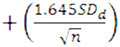 . It is LogCSN,D + 2SDd if design standard SN curves are used (such as those provided in DNVGL-RP-C203).
Figure 4 - Illustrating how the target curve relates to the mean and design standard SN curves
It should be noted that it is not appropriate to calculate the design curve of a small dataset by calculating the mean curve and subtracting two standard deviations because the standard deviation of a small dataset will typically be less than that of the population [6], and so the resulting design curve would be higher than it should be and be unconservative. That approach is only appropriate for large datasets. Another potential source of non-conservatism is sampling errors in the mean of a small dataset; the target curve approach described above is designed to safeguard against sampling errors in both the mean and standard deviation of a small dataset.
5. Analysing the results: the DNV approach
DNVGL-RP-C203 covers two approaches. One is the “engineering approach”, which says that the standard deviation of the test results can be assumed to be the same as that of standard SN curves (and so is ‘known’). It says that engineering judgement should be used to determine this. The alternative is the statistical approach, in which the standard deviation is calculated from the test results (and so is termed ‘unknown’).
A table is provided in DNVGL-RP-C203 Appendix F (derived from complex probability calculations, described in [9] and [12]) which states the number of standard deviations should be subtracted from the mean curve for a given sample size and confidence level to produce a design curve for the test data. This is as high as 9.24SD for an unknown standard deviation with a sample size of 3 and a confidence of 95%.
It also provides guidance on how to justify the use of a standard design SN curve for a new dataset. This uses the same principles as the statistical approach, however it uses a different formulation to determine whether test results qualify to a design curve. In this approach, the Stress Modification Factor (SMF) is calculated for the test results and this relates the design curve for the test results to the standard design SN curve to be qualified to with a particular level of confidence. The approach can be used when the slope of the test data is equal to that of the standard SN curve. The SMF is calculated (from DNVGL‑RP‑C203) as follows:
Where:
| n |
= number of test samples |
| Ni |
= number of cycles for specimen i |
| m |
= slope of the standard design SN curve |
| Δσi |
= stress range for specimen i |
| xc |
= confidence with respect to mean S-N data as derived from a normal distribution. This is equal to 0.674 for a 75% confidence and 1.645 for a 95% confidence. |
| Log a |
= Intercept of the mean standard S-N curve (note this is equal to Log C+2SD) |
| slogN |
= standard deviation of the standard SN curve = 0.2 for the main DNV SN curves. |
Once the SMF has been calculated, it can be used to derive a target curve for the test results as follows [2]:
or equivalently, since the slope of the design curve and target curve are the same by definition, again, the intercepts of the target curve and standard design SN curves can be compared. The intercept of the test result design curve is given by:
6. Worked example
Do the data in Table 2, obtained from full scale resonance fatigue tests on riser-quality girth welds, qualify to BS7608 Class E?
For the dataset of n = 8 test results, regression analysis of the data produces a mean curve with a slope of 2.61 and standard deviation of Log N of 0.169 (note that this is calculated using n - 2 degrees of freedom, because both the slope and intercept are obtained from the regression analysis). The slope is close to that of standard SN curves and the standard deviation is less so it is appropriate to force the slope to equal 3. Now that only one variable is obtained from the regression analysis, the number of degrees of freedom used to calculate the standard deviation becomes n - 1 and this actually decreases the standard deviation to 0.163. The intercept (Log C) with a forced slope of 3 is 12.680.
The aim is to qualify to BS7608 Class E. The intercept of the target curve for a 95% confidence is given by:
Log C = 12.5171+ 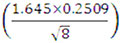 = 12.663.
Since the intercept of the mean curve of the test data is higher than that of the target curve (12.680 > 12.663), the results do qualify to BS7608 Class E using this method.
Using the statistical approach in reverse, the intercept of the design curve is
12.680 - - 2 x 0.2509 = 12.060. The closest standard design SN curve is the Class E design, and so again, Class E would be appropriate for the test data.
Table 2 Sample fatigue test results
| Endurance, N, Cycles |
Stress range, MPa |
| 3,283,120 |
114 |
| 1,662,320 |
145 |
| 3,580,090 |
152 |
| 572,770 |
196 |
| 1,001,520 |
188 |
| 1,274,680 |
177 |
| 1,851,040 |
130 |
| 6,399,260 |
99 |
The alternative is the SMF approach. For the 8 results, and using a 95% confidence, the SMF is equal to 0.92. The intercept of the SMF-based design curve is equal to 12.127 (compared to the intercept of the BS7608 Class E design curve of 12.017). Since the SMF-design curve of the test data is above the BS7608 Class E design curve, the results also qualify to Class E using this approach. The curves are summarised in Figure 5. The intercepts of the curves calculated using the different methods are summarised in Table 3.
Table 3 Summary of Log C intercepts
| Curve |
Log C |
| BS7608 Class E mean |
12.5171 |
| Test data mean |
12.680 |
| BS7608 Class E design |
12.0170 |
| SMF design |
12.127 |
The two approaches produce the same end result (in that the data qualify), but the methods are slightly different. The statistical approach in its basic form aims to compare the mean of the dataset with the target curve, whereas the SMF approach produces a design SN curve for the dataset.
Figure 5 - Results plotted on an SN curve. The BS7608 class E mean and design curves, along with the dataset mean, target and SMF design curves
7. Conclusions
The salient points of statistical analysis of test data, as applied specifically to qualifying the fatigue strength of components to standard design SN curves has been presented and summarised.
- Relevant statistical concepts have been explained in a way accessible to non-experts in statistics.
- ASTM E379 and ISO12107 make recommendations on the number of appropriate tests to carry out when obtaining fatigue test data for various purposes.
- For design data, 12 specimens should be tested. The most practical approach for full scale resonance fatigue testing of girth welded specimens, each containing two welds, is to test with a 75% replication level. This way 2 specimens are tested at each of 3 stress ranges, and even if one weld in each specimen is a runout, the requirements of both standards (E379 and ISO12107) are met.
- The statistical approach to the analysis of fatigue test data involves using regression analysis to calculate a mean of the test data, and this is compared to a target curve, which is a factor above the standard design curve that depends on the number of data points and the level of statistical confidence. It is appropriate for n to equal the total number of specimens if the slope and standard deviation of the test data match that of the standard SN curve.
- The stress magnification factor (SMF) approach produces a design curve from the test data, whose position also depends on the level of statistical confidence and number of test results, n.
8. Acknowledgement
The author thanks Charles Schneider for his valuable input.
9. References
- BS 7608+A1, 2014: ‘Guide to fatigue design and assessment of steel products’, British Standards Institution, London.
- DNVGL, 2016: ‘DNVGL-RP-C203, Fatigue design of offshore steel structures’ Det Norske Veritas, Norway.
- Gurney, T, 1979: ‘Fatigue of welded structures’ Cambridge University press.
- BS5400-10, 1980 ‘Steel, Concrete and Composite Bridges Part 10: Code of Practice for Fatigue’ British Standards institution, London.
- DNV, 1977: Rules for the design construction and inspection of offshore structures, Det Norske Veritas, Norway.
- BS600, 2000: ‘A guide to the application of statistical methods to quality and standardisation’ British Standards Institution, London.
- IIW, 2006: Technical note for CENTC54, WG C Subgroup ‘design criteria’- derivation of fatigue test factors to be applied in the design by experiment part of EN13445, May 2006.
- Schneider C R A and Maddox S J, 2003:‘Best practice guide on statistical analysis of fatigue data’. TWI Core Research report 13604.01/02/1157.02, July. Also issued as IIW document number Doc IIW-XIII-WG1-114-03
- Ronald K O and Lotsberg I, 2012: ‘On the estimation of characteristic S-N curves with confidence’ Marine Structures, vol 27, pp 29-44.
- ASTM E379-10: ‘Standard practice for statistical analysis of linear or linearized stress-life (S-N) and strain -life (ε-N) fatigue data’, ASTM International
- BS EN ISO12107, 2003: ‘Metallic materials - fatigue testing - statistical planning and analysis of data’ British Standards Institution, London.
- Lotsberg, I and Roland R O, 2011: ‘On the derivation of design S-N curves based on limited fatigue test data’ OMAE2011-49175.