Davide Kleiner, Chris Edwards and Ruth Sanderson
R Kazys, V.Cicenas, R Raisutis, E Jasiuniene and K Barsauskas
Ultrasound Institute, Kaunas University of Technology, Lithuania
Paper published in I Mech E Seminar: Storage Tanks, London, 16 June 2005.
Synopsis
Large storage tanks containing hazardous liquids such as oil, oil-derived products and food processing liquids are common throughout the world. Corrosion in the tank floor is a serious environmental and economic risk.
TWI is managing a European CRAFT project called TANKINSPECT to overcome the drawbacks of current inspection practices. By placing Long Range Ultrasonics (LRUT) sensors outside the tank and using reconstructive tomographic techniques there is potential for carrying out an inspection of the whole tank floor without the requirement of emptying and cleaning the tank or operator entry inside the tank.
The project, a €2million Framework 6 project, started in March 2004 and is due to finish in February 2005. The research carried out so far has already shown very promising results both on the numerical modelling and the practical inspection development sides, making the consortium very confident that a working product will be successfully delivered by the end of the project.
1 Introduction
Numerical modelling of ultrasonic wave propagation has been carried out in structures representative of storage tank floors. The floors are constructed from overlapping lap welded steel plates. The attenuation of waves propagating in lap welded steel plates loaded by diesel and sitting on wet sand has previously been reported [1] . The paper presents results of 3D modelling using finite sized transducers to generate waves at an angle of incidence to a lap weld.
2 Investigation of propagation of SH and S0 mode plate waves in unconstrained tank floor with weld by 3D numerical modelling
2.1 Description of 3D finite element model
The aim of the simulation is to investigate the properties of waves of different polarization propagating in structures made of several plates welded together. The lap welds as well as complex interaction of the plates with surrounding acoustic media (oil on one side and soil on another) makes the overall structure irregular. Practically, the only means to obtain realistic solutions is the finite element simulation by using 3D solid or coupled solid-acoustic models.
2.1.1 Geometry of the model
The 3D finite element computational model composed of linear elastic elements has been built using ANSYS and LSDYNA finite element codes. ANSYS has been used to generate the volumes and to perform the meshing of the model. The problem is then solved in LSDYNA environment. The geometry of the model generated in ANSYS (APDL internal programming language) is fully parametric. Two models have been investigated:
- Two overlapping plates welded together, Figure 1;
- Three overlapping plates, Figure 2.
The parameters used for both sample calculations are presented in Table 1.
Table 1. The parameter values used in the calculation
| | H,
[mm] | B,
[mm] | b 1,
[mm] | b C ,
[mm] | L 1,
[mm] | L 2
[mm] | L seam ,
[mm] | L overlap ,
[mm] |
|---|
| Two welded plates |
6 |
250 |
50 |
0/-100 |
250 |
250 |
6 |
80 |
| Three welded plates |
6.17 |
249 |
24.7 |
24.7 |
249 |
249 |
6 |
39.1/80
(L3) |
The size of an element is selected based on the consideration that 20-30 elements should be used per wavelength.
Element type 99 of LSDYNA program has been used in the model. The element is intended for vibration studies carried out in the time domain. These models may have very large numbers of elements and may be run for relatively long durations. The purpose of the element is to achieve substantial CPU savings. This is achieved by imposing strict limitations on the range of applicability, thereby simplifying the calculations:
- Elements must be cuboids; all edges parallel to the global x,y,z axes;
- Small displacement, small strain, negligible rigid body rotation;
- Elastic material only.
With this element, the performance of the model is similar to the fully integrated solid, however the performance is even better than that of traditional constant strain element. Single element bending and torsion modes are included, so meshing guidelines are as for fully integrated solids - e.g., thin structures can be modeled with a single solid element through the thickness if required.
In order to satisfy the requirements posed upon the element geometry, the welded seam has been modeled as a line of elements with a rectangular cross section. It appears reasonable to expect that the micro-geometry of the cross-section will not substantially influence the simulation results as the wavelengths investigated here are considerably (about 6-7 times) larger.
2.1.2 Material model
The whole assembly is assumed to be a homogeneous elastic steel structure and is modeled in LSDYNA by using *MAT_ELASTIC model as presented in Table 2.
Table 2. The parameters of *MAT_ELASTIC model, where ρ is mass density, E is Young's modulus, σ is Poisson's ratio.
| $ STEEL elastic |
|---|
| *MAT_ELASTIC | | |
|---|
| $MID |
ρ |
E |
σ |
| 1 |
7800 |
2.0533E+11 |
0.29 |
From these values, the longitudinal and transverse (shear) wave velocities are c L =5900m/s, c T =3190m/s. The shortest expected wavelength at 50kHz frequency excitation is 63.8mm and by taking 25 elements per wavelength we have an element size of 2.552mm. So for the 250x500x6mm plate we need 98x196x3=57624elements or 78012 nodes. If local behavior of the wave near, say, defect edges is to be investigated where wave transformations and generation of higher frequency components may take place, a finer mesh would be required.
2.1.3 Boundary conditions
The structure for ultrasonic wave propagation simulation is unsupported, as is the usual practice in modelling of problems of high-frequency vibration. The weld in the model (see L seam in Figure 1) indicates the ideal connection (coincidence) of nodes. The overlapped region (see L overlap in Figure 1) of the two plates can also be treated as a free boundary. The reason is that the amplitudes of the investigated waves are small enough to avoid interaction between the plates because of the small gap which exists in reality between the plates in non-welded regions.
2.1.4 Wave mode excitation
The ultrasonic wave is excited by means of a piezoelectric transducer (PT). Due to the inverse piezoelectric effect phenomenon the PT deforms under the influence of an applied external electric field. The simplest approximation of the phenomenon may be presented by means of the equivalent force diagram, Figure 3. The deformation excited in the PT is defined as
S J = d iJE i,
where d iJ is the piezoelectric strain modulus ( i=1,2,3 correspond to the three longitudinal directions of possible application of an electric field E i ), S J - the strain tensor presented in Voigt's notation ( J=1,2,3 correspond to the three longitudinal components of the strain and J=4,5,6 - to shear strains in coordinate planes xy, xz, yz correspondingly). In approximate evaluations it is usually assumed that the deformation mode of the PT under the electric field E i applied in direction i is determined by the largest value
. The stresses caused by the piezoelectric effect phenomena can be conveniently presented as
T J =
d iKc KJE i =
e iJE i , where
e iJ is the piezoelectric coefficient
e iJ =
d iKc KJ , and
c KJ is the stiffness tensor determined under constant electric field. The scheme of stresses in the plate created by means of its interaction with the PT excited by the electric field component
E l is presented in
Figure 3. The excitation waveform is a 50kHz sinusoidal tone burst.
2.1.5 Exciting waves propagating at an angle to the boundary
The transducers shown in Figure 3 are divided into sub elements. If these are driven uniformly, waves propagating in the direction normal to the boundary of the plate are generated. The transducer elements can be driven with phase delays to generate waves at an angle.
| a) |
b) |
 |
 |
| Fig. 3. Free body diagram of the excitation of shear (a) and longitudinal (b) ultrasonic waves. Shear (a) or longitudinal (b) stress components are excited in the piezoelectric transducer as a consequence of the electric field component E1 and causes the corresponding interaction stress to be created in the plate |
2.2 Propagation of S H and S 0 mode waves in unconstrained damaged floor
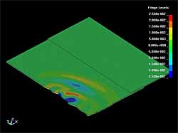
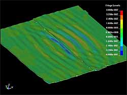
The propagation of the S 0 mode Lamb waves has been investigated in previous stages of the project. The investigation of the interaction of these waves with the lap joint weld has been also performed using 2D models. [1] The objective at the present stage of modelling was to investigate the features of the S 0 and S H plate waves interaction with the weld and defect in 3D. Figure 4 to Figure 7 present the distribution of acoustic field in the welded or defected plate at different time instances with different excitation conditions. In these figures the amplitude of the particle velocity vector is denoted by the colour coding. The vertical particle displacement can be observed as 'surface wave' in 3D images. Figure 4 presents the interaction of S 0 mode Lamb wave with the lap weld. It can be seen that after the interaction with the weld, the S 0 mode is partially reflected, transmitted and mode converted. A 0 Lamb waves are generated in the forward and backward directions. Figure 5 also shows the case when the S 0 mode Lamb wave was generated at an angle with respect to the weld. The waves after the interaction have a similar character, but the A 0 Lamb is generated at an angle to the weld.
| a) |
b) |
 |
 |
| Fig. 4. Acoustic field of S0 Lamb wave before hitting the lap joint weld (a) and after interaction with weld (b) |
| a) |
b) |
 |
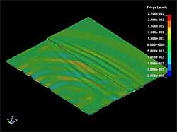 |
| Fig. 5. Acoustic field of S0 Lamb wave before hitting the lap joint weld (a) and after interaction with weld (b). The waves are generated at 30° with respect to the weld |
| a) |
b) |
c) |
 |
 |
 |
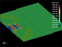
| Fig. 6. Acoustic field of SH wave before hitting the lap joint weld (a), at the instant when S0 Lamb wave hits the weld (b) and after interaction with weld (c) |
The propagation of the S H waves is more complicated. Due to the finite dimensions of the transmitter some S 0 waves are generated from the transducer edges in addition to the pure S H mode ( Figure 6a). S 0 mode Lamb waves are faster then S H mode Lamb waves, so they hit the weld first ( Figure 6b) and generate A 0 Lamb waves. Later the slower S H wave reaches the weld and generates additional A 0 waves ( Figure 6c). It can also be observed that the amplitude of these secondary A 0 Lamb waves is less in the central part. Possibly, generation of the mode converted A 0 Lamb waves from the S H mode waves is stronger when they hit the weld at an angle.
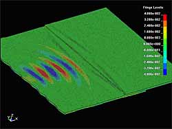
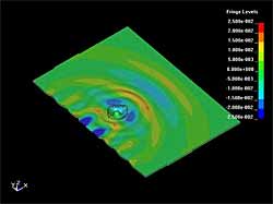
Figure 7 shows the interaction of the S 0 and S H mode waves with a disk shape defect. The defect diameter is 50mm and it extends through half the plate thickness. It can be seen that in both cases the defect is the source of A 0 Lamb waves which propagate almost uniformly in all directions. The particle displacement and particle velocity in the defect region have much higher amplitude, so it can be assumed that the defect acts as a virtual transmitter. If the plate is covered by some liquid medium, this virtual transmitter (defect) should generate acoustic waves propagating into the liquid. The directivity of this generation of course depends on the defect geometry. It can be observed that the S 0 Lamb wave propagates through the defect almost without decay, while the S H mode has some amplitude decay in the region after the defect. This can be explained by the fact that the wavelength of S 0 mode is almost twice the diameter of the defect, while the S H wavelength is comparable with the size of the defect. So, the S 0 Lamb wave is diffracted around the defect and decay of the amplitude cannot be observed.
| a) |
b) |
 |
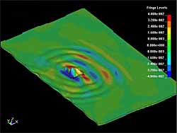 |
| Fig. 7. Interaction of the S0 (a) and SH (b) waves with the disk shaped defect, 50mm diameter (0.5 wall thickness) |
2.3 Propagation of SH and S0 modes in 3D lap joints
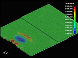
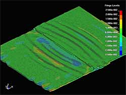
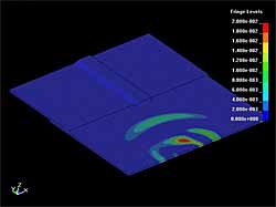
The interaction of the S 0 mode Lamb wave with the 3D lap joint is shown in Figure 8 to Figure 9. In all cases the waves were generated at 30° with respect to the normal of the plate edge. Figure 8 shows the distribution of y component of particle velocity before and after hitting of the weld by the S 0 mode wave. The essential decay of the wave amplitude can be observed after the joint. The results presented in Figure 9 demonstrate that due to the interaction the A 0 mode Lamb wave is generated. In Figure 10 to Figure 11 similar results obtained with the S H mode wave are presented. Comparison between the S 0 and S H mode waves demonstrates that the S H mode passes the lap joint with lower attenuation than the S 0 mode. It can be seen also that the amplitude of the secondary A 0 wave is smaller than for the S H mode wave. For more detailed estimation of the wave attenuation caused by the weld, the waveforms of corresponding y and x components of particle velocity were acquired at the points shown in Figure 12. Comparison of amplitudes of the waveforms before the weld (point P 1) and after (point P 2) have shown that the attenuation of the S 0 mode is approximately 7dB and that of the S H mode wave is about 11dB. This estimation (attenuation of the S H mode > S 0 mode) contradicts the conclusions made from the 3D images. This can be explained by the fact that the point based estimations depend on the selected point, because the field is very non-uniform due to interference of different reflections. Nevertheless, the obtained value in general coincides with the results of 2D modelling and experimental investigations presented previously. [1]
| a) |
b) |
 |
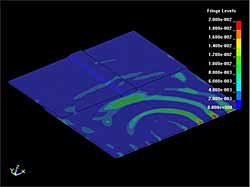 |
| Fig. 8. Distribution of the y component of the particle velocity of S0 Lamb wave before hitting the 3D lap joint weld (a) and after interaction with the weld (b) |
2.4 Experimental results
Experiments have been carried out with a linear array of shear transducers dry coupled to the edge of a steel plate. Propagation distances of over 100 metres have been achieved.
3 Conclusion
Both theoretical modelling and experiments indicate that Long Range ultrasound can be used to inspect the bottom plates of storage tanks.
4 References
- R.Kazys, L.Mazeika, A. Demcenka ,V. Cicenas and Ruth Sanderson, 'Condition monitoring of large oil and chemical storage tanks using guided waves' Insight 2004