Yanhui Zhang
Fatigue life of a component is composed of two stages: crack initiation and crack propagation. Fracture mechanics is the method used to predict crack growth life. It is particularly useful for components which contain defects or a crack. The main applications of fracture mechanics based fatigue analysis include determination of the maximum tolerable initial flaw size (often involving welds) for design life, calculation of crack growth life with a known or assumed crack size and planning of inspection intervals. To predict crack growth accurately using this method, it is essential to conduct tests to obtain the fatigue crack growth rate (FCGR) of the material under appropriate environmental conditions.
FCGR is often expressed as a function of stress intensity factor range, ΔK, in terms of the Paris power law:
da/dN = A ΔKm [1]
where da/dN is crack growth per cycle, ΔK is a function of stress range, crack size and specimen geometry, A and m are material constants which need to be determined by carrying out fatigue crack growth tests.
There are two well recognised standards for conducting FCGR tests: ASTM E647 (1) and ISO 12108 (2). They are largely in accord, but there are some small differences between the two. Examples of such differences include the specification of the parameter C, which is the magnitude of load drop during a decreasing ΔK FCGR test (-0.08mm-1 in ASTM E647 while -0.1mm-1 in ISO 12108) and the definition for the crack growth threshold, ΔKth: 10-7mm/cycle in ASTM E647 while 10-8mm/cycle in ISO 12108.
FCGR tests require use of standard specimen geometries which include compact tension (CT), single edge notch bend (SENB), single edge notch tension (SENT) and centre crack tension (CCT) specimens. Both ASTM E647 and ISO 12108 accept these specimen geometries and provide the K solutions. Figure 1 shows the geometries of SENB and CT specimens which are more often used than the other two. Compared to the SENB specimen, the CT specimen has the advantage of being more economical in material which can be important when the material sample is limited. However, machining of such a specimen is more expensive. Another advantage with the SENB specimen geometry is that it is easier to set up a test in a corrosive environmental chamber.
Standards (1, 2) specify the size requirements for specimen, notch and pre-crack. Notch is often produced by electrical discharge machining (EDM) and pre-crack is introduced by cyclic loading. It is important to ensure that the last maximum K (Kmax) in pre-cracking is less than the Kmax used at the start of a FCGR test. To achieve this, pre-cracking is often conducted at a stress ratio lower than that used in the subsequent FCGR test.
Crack growth rates are often monitored using either direct current potential drop (DCPD) or compliance methods. The measurements can be automatically logged using a computerised logging system and converted to crack length using a closed form analytical expression. Figure 2 shows the FCGR set up for a SENB specimen where DCPD probe wires and current leads are attached to the specimen for crack growth monitoring. Crack growth measurements using a microscope is also sometimes used.
Fatigue crack growth (FCG) tests can be carried out under either increasing or decreasing ΔK. In the former, the maximum and minimum loads are kept constant so ΔK increases with increasing crack size. For the latter, ΔK is decreased in steps, which is specified by the parameter C, and the reduction of Kmax, shall not exceed 10% of the previous maximum stress-intensity factor to avoid crack growth retardation phenomenon.
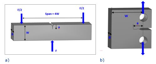
Figure 1 Two types of common specimen geometries for FCGR testing: a) SENB; b) CT.
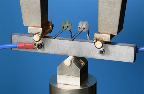
Figure 2 FCGR test set up for a SENB specimen in air.
Stress ratio, R, is defined as ratio of minimum to maximum stresses in a cycle. It has a strong effect on FCGR of a material. FCGR tests are often conducted under a constant R. For welds, FCGR tests are often conducted at a stress ratio ≥0.5 to account for the possible high tensile residual stresses present in welds which may be relaxed when a specimen is extracted from a component. This is in accordance with BS 7910 (3) which is a fracture mechanics based guide to methods for assessing the acceptability of flaws in metallic structures. Another approach is to adopt a constant Kmax so that R varies during a test: higher at low ΔK but low at high ΔK. This enables obtaining FCGR data at high ΔK level without significantly violating the remaining ligament criterion (to be described later). Furthermore, it is generally found that stress ratio has a strong effect on FCGR in the low ΔK regime but small effect in the high ΔK regime. Because of high tensile residual stresses (RS) in welds, a high effective stress ratio (combination of applied stress range and RS), eg, 0.7, is possible in this regime. Therefore, use of a constant Kmax produces more conservative FCGR in the region near the ΔKth.
For components containing a weld, fatigue cracking often initiates at the weld toe and its growth may propagate through different microstructures. Therefore, the effect of microstructure and crack growth path should be considered by choosing the appropriate notch position. For a single-sided girth weld in a pipeline, a fatigue crack may initiate from either outside or inside of a pipe and the crack may propagate through weld metal (WM), heat affected zone (HAZ) or parent metal (PM) depending on weld profile and service conditions. Figure 3 schematically shows the possible notch positions for consideration. Experience has shown that, for FCG in either the PM or WM, notching from the OD and ID gives similar FCGR data.
The notches shown in Figure 3 are in the NQ orientation according to the notation specified in ISO 15653 (4). Another option for testing a weld can be in the NP orientation where the notch is through the plate/wall thickness and the crack propagates along the weld direction.
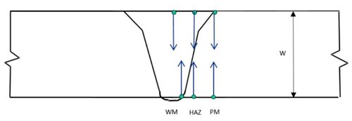
Figure 3 Schematic showing three notch positions from either outside or inside the surface of a girth welded pipe.
A notch is often introduced using electric discharge machining (EDM), with a wire diameter typically of 0.2mm.
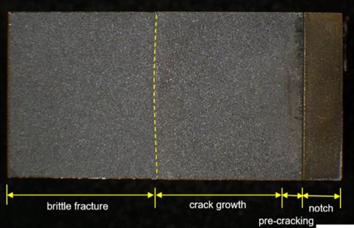
Figure 4 Example of fracture surface of a FCG test specimen, showing the final crack front before brittle fracture.
FCGRs often exhibit a large scatter in the low ΔK regime but relatively small in the high ΔK regime (5). The data scatter for the former is associated with the sensitivity of many variables in this regime, including microstructures, residual stresses, changes in crack tip geometry (crack branching), mechanisms associated with crack closure and environment. For each set of tests, it is recommended to conduct at least three FCGR tests: one under increasing ΔK and two under decreasing ΔK to obtain FCGR data over a large range of ΔK. Depending on specimen size, it would be a good practice to start a decreasing ΔK test at ∿400N/mm3/2 and an increasing ΔK at ∿300N/mm3/2 to include an overlap between the two.
After a test is completed, the specimen is broken following immersion in liquid nitrogen (depending on the material) to reveal the fracture surfaces. One example is shown in Figure 4. Nine crack length measurements across the crack width with an even spacing are carried out to obtain the average final crack size which is used to calibrate the crack sizes estimated by either the DCPD or compliance method.
Afterwards, it is important to check the validity of the FCGR data obtained. The Standards (1, 2) specify several validity criteria including crack front curvature and minimum un-cracked ligament (small plastic deformation ahead of a crack). In regards to the requirement for the minimum un-cracked ligament, the yield strength of the metal, where a crack propagates through, is required. This criterion only needs to be checked for the data obtained at high Kmax. Experience indicates that, when this criterion is not significantly violated, the invalid data follow reasonably well with the extrapolation of the valid data to higher ΔK levels and could still be acceptable.
In corrosive environments, FCGR strongly depends on loading frequency which in turn depends on ΔK magnitude. For testing in a marine environment for offshore application, a loading frequency of 0.2Hz is often applied since it represents wave loading frequency. For some applications, for example, lateral buckling of offshore pipelines, the loading frequency is typically very slow. Frequency scanning (FS) testing is often used to determine the effect of loading frequency on FCGR in corrosive environments. In this type of test, ΔK is kept constant while the loading frequency is gradually changed, more often decreased, at regular steps after a certain crack extension (about 1mm), until a saturating loading frequency is reached at which the FCGR achieves the maximum FCGR. The crack growth rate at any particular loading frequency is determined by calculating the slope in a plot between crack length and number of cycles. To avoid any possible transient crack growth rate data being included in the analysis, the crack growth data corresponding to the initial crack extension after each change of loading frequency is often excluded from the analysis. In the meantime, FCGR tests are carried out in the same environment at a fixed loading frequency, typically between 0.1-0.3Hz. The loading frequency accelerating factor (LFAF), defined as the ratio of the FCGR at a particular lading frequency, (da/dN)f, to the FCGR at the fixed loading frequency, is calculated. The maximum LFAF (MLFAF) value is often conservatively applied to FCGR data obtained at the fixed loading frequency. To appropriately account for effect of loading frequency on FCGR, several frequency scanning tests, each at a different ΔK level, are required.
FCGR testing in corrosive environments are required to be carried out in specialised testing facilities for environmental control such as partial pressure, pH value of solution, temperature, aqueous solution, oxygen content in solution, test gas composition, etc. Pre-soaking is required to ensure a specimen is fully charged before testing.
DNVGL F108 (6) recommends a minimum four days soaking period in aggressive environments for offshore structures, such as in H2S. However, since a specimen is continuously exposed to the environment during testing, and for specimens with a crack, it is the hydrogen content in the crack tip region that will influence the FCGR behaviour, the actual pre-charging period could be less than four days.
Once the FCG tests and post-test examination have been completed, statistical analysis of the data are required to determine the material constants in Eq. 1. Both ISO 12108 and ASTM E647 recommend to use either the Secant or polynomial methods. The Secant method is more often used because of its simplicity. It involves calculating the slope of the straight line connecting two adjacent data points on the crack size, a, versus N curve.
For the FCGR data obtained under different conditions, for example, notch position, welding procedure, microstructure, material strength and component dimensions, statistical analyses should first be carried out to determine whether the data under different conditions, belong to the same population, ie having the same FCGR curve, or whether the difference between the two sets of results is significant. This can be carried out using the guidance on statistical analysis of fatigue data (7). If there is no significant difference in FCGR for a given significance level, the data can be combined to form one population in the following regression analysis.
FCGR data often exhibit two stages as shown in BS 7910. The FCGR data obtained need to be separated into two groups by setting up a ΔK or FCGR value corresponding to the transition which is often visually judged. The data below and above the transition point are in the stages A and B, respectively. Regression analysis is carried out by setting ΔK as variable to determine parameters A and m. The m value thus determined is called the natural slope. As the database in a particular testing programme may be relatively small, it is sometimes assumed to be identical to that given in BS 7910. This slope is called the forced or fixed slope. Standard deviation, SD, should be determined. When the data base is relatively large, greater than about 60 data points, the design parameter A can be simply calculated as:
log(Adesign)=log(Amean)+2SD [2]
The FCGR curve with Adesign corresponds to a small exceedance probability, 2.5%. This is the FCGR curve often used in fracture mechanics based fatigue design or for the planning of inspection intervals.
For more information, please email contactus@twi.co.uk.
References
- ASTM E647-13a, 'Standard test method for measurement of fatigue crack growth rates', ASTM International, USA, 2013.
- ISO 12108, 'Metallic materials - Fatigue testing - Fatigue crack growth method', International Standard Organization, 2018.
- BS 7910, 'Guide to methods for assessing the acceptability of flaws in metallic structures', British Standard Institution, London, UK, 2019.
- ISO 15653, 'Metallic materials - Method of test for the determination of quasistatic fracture toughness of welds', International Standard Organization, 2010.
- King R N, 'A review of fatigue crack growth rates in air and seawater', HSE Report OTH 511, 1998.
- DNVGL-RP-F108, 'Assessment of flaws in pipeline and riser girth welds', DNV GL, October 2017.
- Schneider, C R A and Maddox S, 'Best practice guide for statistical analysis of fatigue data', The Welding Institute, 2003.