Mon, 28 June, 2021
WrapSense is an InnovateUK collaborative project between Direct-C, TrackWise and TWI, aiming to research, develop and validate novel technologies for hydrocarbon leakage detection. The technology is based on a novel, highly sensitive nano-composite coating material capable of detecting even the slightest concentration of liquid hydrocarbons coming into direct contact with it. This makes it a highly effective technology for detecting leakages in oil and gas and aerospace applications.
After the sensors’ installation and successful webinar presentation, this press release summarises the results for the three month exposure test.
Initial Test Data March 2021
The weather variables along with the WrapSenseLD data were recorded over a 3 month-period starting from 1st of January to 31st of March. The figure below (Figure 1) shows the 10 x 1m WrapSenseLD sensor’s data. The steep slope indicates the sensors testing via exposure to hydrocarbons (similar to the small-scale testing), applicable to Sensor 0 to Sensor 4. The remaining sensors (S5 to S9) are untested.
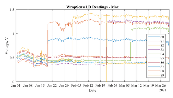 Figure 1. WrapSenseLD 3-month readings
Similarly, the figures below (Figure 2a-2d) shows the recorded weather variables. Cold temperatures were recorded during January and the first half of February, followed by an increase towards mild temperatures until mid-March. The last weeks recorded a rise in temperature reaching beyond 20°C. The relative humidity seems to commence around 100% saturation at the start of the day, followed by a steep drop to 80%, 70% and even 60% during the day. In addition, several rain episodes were recorded predominantly over the winter months and a good part of Mid-March. Finally, the average wind speed is registered around 20 kph with some events exceeding 40 kph.
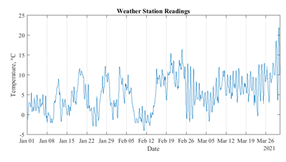 Figure 2a. Temperature recordings - 3 months
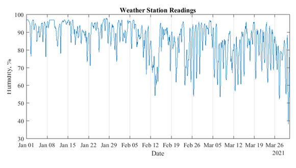 Figure 2b. Relative humidity recordings - 3 months
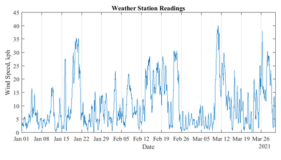 Figure 2c. Wind speed recordings - 3 months
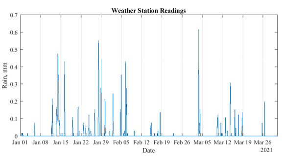 Figure 2d. Rain recordings - 3 months
WrapSenseLD’s Performance Assessment
In order to assess the sensor’s performance against the environmental exposure, the following methodology was proposed:
- Obtain the periodicity of WrapSense data (if any) via autocorrelation
- Obtain the periodicity of weather data via autocorrelation
- Perform a cross-correlation of periodic data between WrapSense and weather data
- Conduct a delayed response correlation for non-periodic data
Cross-correlation is a technique that measures the similarity between a vector x and shifted (lagged) copies of a vector y as a function of the lag [6]. Where the y vector is a copy of the x vector, it is denominated as ‘autocorrelation.’ Conversely, for independent variable vectors x and y is denominated ‘cross correlation.’
In order to compare the entire WrapSenseLD sensor’s data, the tested sensors are post processed by eliminating the voltage increase due to the sensor exposure. This is done by subtracting the voltage values after the test, for the voltage value immediately before the test. The figure below (Figure 3) shows the post processing example for Sensor 4:
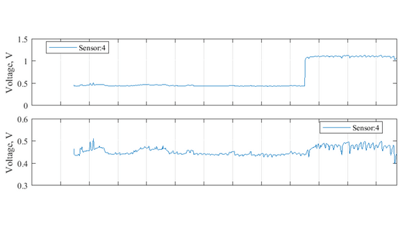 Figure 3. Sensor 4 normalisation example
WrapSenseLD Autocorrelation
The autocorrelation is performed in Matlab using the “xcorr” function. Since autocorrelation values are symmetric, only the positive lag is indicated. Figure 4 shows the autocorrelation values for the tested sensors (S0 to S4). It can be observed that autocorrelation values clearly peaks every 0.87 days. Conversely, the autocorrelation results for the untested sensors (S5-S9 right) are less evident. Nonetheless, the average period for the untested sensors are 0.95 days. Both autocorrelation results indicates that the sensor’s data is daily periodic.
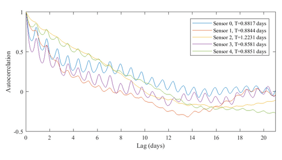 Figure 4. WrapSense tested sensors autocorrelation
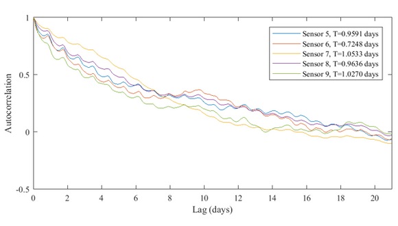 Figure 5. WrapSense untested sensors autocorrelation
Weather Data Autocorrelation
By employing the same cross-correlation function, the autocorrelation values are obtained for the weather variables. Figure 6, below, shows the results and periodicity values for temperature, humidity, rain and wind speed. For the temperature series, it is evident that the temperature oscillates daily following the day/night cycle (period equal to 0.9994 days). Moreover, the plot shows a secondary cycle from day 0 to day 18; this might indicate a change in temperature due to the season. Full year-long data will provide the seasonal cycling of temperature. Similarly, the relative humidity behaves on 0.9994 days of periodicity. Unlike the temperature variable, the humidity does not seem to have a secondary cycle due to the seasonal effect. It can be inferred that the autocorrelation factors oscillate constantly between -0.2 and +0.4.
In addition, the results indicate that either rain or wind speed are not periodic variables. The rain’s data autocorrelation values are close to zero for any lagged day. Similarly, the wind speed autocorrelation randomly oscillates during the lagged days with no clear period identification.
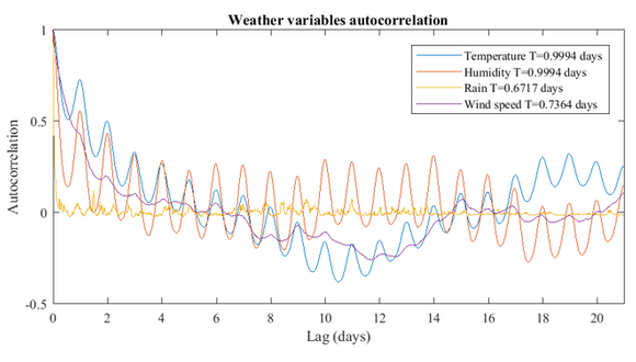 Figure 6. Weather data autocorrelation
WrapSenseLD and Weather Data Cross Correlation
Before operating the cross-correlation function, the data shall be synchronised to obtain the same vector’s length. The WrapSenseLD data is recorded approximately every 70 minutes, whereas the weather data is sampled every 15 minutes. The synchronisation is performed using the “synchronise” function in Matlab for “timetable” data types. The following figures show an example of WrapSenseLD sensor 8 data against temperature and humidity from 26 February to 5 March. It is important to note that the series are plotted in different vertical axis for better representation. The data used for the analysis has been processed by subtracting the mean value of the entire data set; this process is applied to WrapSenseLD, temperature and humidity data.
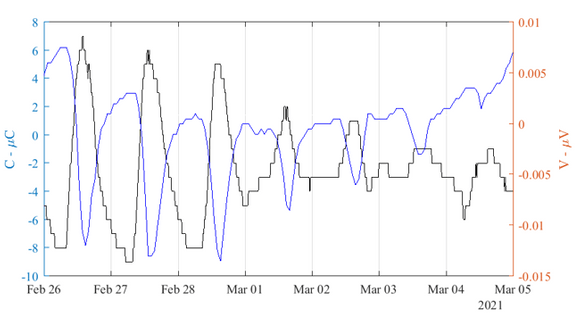 Figure 7. WrapSense and temperature – time series
For the temperature cross-correlation, it is clear that the WrapSense performance is out-of-phase. This means that peak temperatures, normally around 2pm, correlate with drops in the sensor’s voltage, featuring a minor delay between peaks. However, it is remarkable that the start of the temperature increase, for instance around 9am, does not necessarily correlate with the start of the drop in the sensor’s voltage.
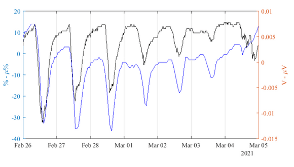 Figure 8. WrapSense and humidity – time series
In contrast, WrapSenseLD’s voltage cross-correlation with relative humidity is in-phase with the humidity drops that occur during the day. Moreover, the shape of the voltage signal is similar to the relative humidity. For example, humidity’s behaviour is characterised by a steep drop (typically around 9am) followed by a steady recovery during the day and a stabilisation period overnight. This behaviour is mirrored by the voltage signal featuring the aforementioned steep drop, steady recovery and stabilisation.
Although some performance variations has been identified, further analysis is required. For example on 4 March, the voltage signal increased regardless of the mild temperature variation and absence of humidity drop. In order to obtain an overall behaviour, the cross-correlation factors are investigated and shown in Figures 9 and 10.
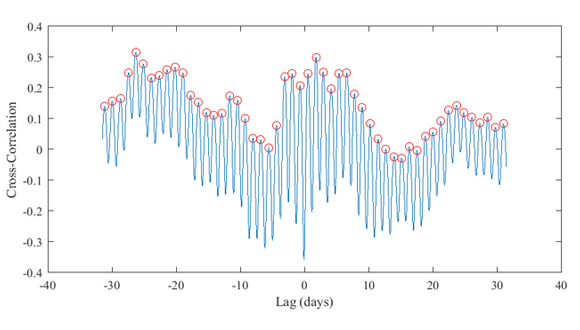 Figure 9. WrapSense and temperature - cross correlation
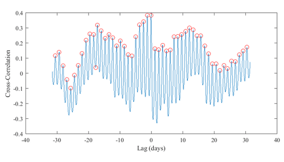 Figure 10. WrapSense and humidity - cross correlation
Figure 9 shows the cross-correlation values for temperature and figure 10 shows humidity. The cross-correlation periods are 1.21 and 1.19 days respectively. It is evident that the correlation is periodic with values oscillating on a constant band of +/- 0.4.
Delayed Response of Non-Periodic Variables
From the weather autocorrelation results, rain and wind speed are not periodic variables. In order to evaluate a possible delayed response, the following methodology is proposed:
- Compute the sensor moving daily average
- Evaluate the signal’s response 3 days before and after the non-period event
- Verify significant changes in the sensor’s daily average
The rain events are selected as recording more than 0.3mm of rain during an hour, the selected events are shown in the table below:
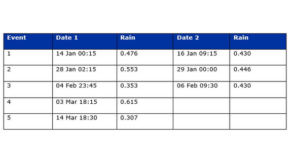
Figure 11 shows the results for Event #5; the top part represents the normalised sensor’s voltage signal and the bottom shows the corresponding rain event. It can be observed that the sensor’s average keeps oscillating based on the temperature and humidity effects but does not appear to be altered by the rain events. The mean values remain following the previous trends.
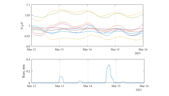 Figure 11. Rain event #5 and delayed response analysis
Finally, it is difficult to assess the wind speed effect on the sensor’s performance as these are non-periodic and volatile, which means the sensor will be in contact with air rather than water or condensation. From an installation perspective, the sensors have been able to withstand 40 kph winds without compromising integrity (sensor is still operative) and detectability.
The Wrapsense Project is funded under InnovateUK Project Number 105611