Limit Load for Embedded Flaws in Pipeline Girth Welds Pt II

Analysis of Limit Load for Embedded Flaws in Pipeline Girth Welds: Part II: Development and Validation of New FEA Models

Tyler London and Isabel Hadley*
TWI Ltd, Granta Park Great Abington, Cambridge, CB21 6AL, UK

Presented at ESIA13, 13th International Conference on Engineering Structural Integrity Assessment, 19 and 20 May 2015, Manchester, UK

This paper concerns the calculation of the reference stress (or limit load) for use in Engineering Critical Assessment (ECA) of circumferential embedded (buried) flaws in pipes.

An FE model of a bend test carried out on a 36in (914mm) OD pipe containing a circumferential embedded flaw has been developed and compared against the published test results. Two analysis methods were adopted: a spreading plastic zone method and a J-based method. The latter requires direct elastic-plastic FE modelling of the flawed component, then forcing a fit between an Option 3 FAD (produced by FEA) and the Option 1/Option 2 FAD as defined in R6 (BEGL, 2001 ^[1]) and BS 7910 (BSI, 2013 ^[2]). Use of a J-based FAD is shown to improve the analysis compared with use of the analytical equations in R6 ^[1] and BS 7910 ^[2].

A companion paper (Hadley et al [3]) describes the background to the limit load solutions in R6 and BS 7910, and compares them with results of an FE analysis of a 400mm OD pipe.

1. Introduction

The challenges associated with analysis of the limit load associated with embedded circumferential flaws in pipes are outlined in part I of this paper ^[3]. As part of an effort to validate and, where possible, improve the solutions available in the R6 and BS 7910 procedures, attempts were also made to re-analyse the results of a pipe bend test carried out in Canada in the 1980s.

This paper includes:

• A review of the use of FEA methods to describe plastic collapse in flawed components
• An overview of two published full-scale tests on pipelines containing embedded circumferential flaws
• Results of an analysis of one of the full-scale pipe bend tests, using two different approaches (spreading plastic zone and a J-based method)
• A preview of ongoing work based on a tool for rapid generation of FE meshes for cracked bodies

2. Reference Stress/limit load Calculation using FEA

2.1 General

There are two main methods to determine collapse (limit) loads of a flawed structure from FEA. The first, referred to as the “spreading plastic zone” approach in this paper, is in line with traditional continuum mechanics theory and assumes an elastic- (or rigid-) perfectly plastic material behaviour. As the applied load increases, a plastic zone develops at the crack tip and spreads through the uncracked ligament, leading to a condition of “local collapse” when the plastic zone snaps through the remaining ligament. The second, a “J-based” method relies on the calculation of the J-integral of the flaw in the structure, and requires the full stress-strain curve (including strain hardening) for the material model.

2.2 Spreading plastic zone method

A lower bound limit load can be calculated by applying small displacement theory with an elastic-perfectly-plastic material model. The limit load is obtained from the point at which yielding spreads across the uncracked ligament. In finite element software, this is done by applying the loads incrementally and proportionally until the plastic zone spreads from the crack tip through the thickness of the section containing the flaw. In Abaqus, the load increment at which local collapse occurs can be determined by monitoring the equivalent plastic strain variable (PEEQ) or the active yielding (AC YIELD) variable. For surface-flaws, this definition is straight-forward as there is only one ligament (or crack tip plastic zone) to consider. However, for embedded flaws, there are two, potentially different sized, ligaments. If one ligament is significantly smaller than the other, then taking the limit load as the load causing the plastic zone to snap through the smaller of the two ligaments may result in an under prediction of the limit load. This is because relatively little yielding of the local section containing the flaw will likely have occurred.

2.3 J-based limit loads

An alternative to the spreading plastic zone method is to determine the limit load based on reference to the crack driving force estimation schemes that the failure assessment diagrams are based upon. Three methods are detailed below.

2.4 API 579 approach

This approach for calculating J-based limit loads is specified in Section B.6.4.3(e) of API 579 (API, 2000 ^[4]) and in a slightly different form in equation B.1.89 (Appendix B1.7.4) of API-579-1/ASME-FFS-1 (API/ASME, 2007 ^[5]). Let:

(1)

where P_ref is determined from the following relationship:

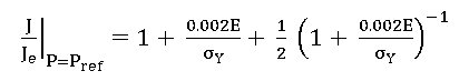
(2)

where J is the total value of J determined from an elastic-plastic analysis of the flawed component; J_e is the elastic J-integral determined from a linear elastic analysis or by converting the mode-I stress intensity factor from a suitable codified solution; P is applied load (or stress); and P_ref is the reference load (or stress) defined as the load at which the ratio J/J_e reaches the value defined by Equation (2).

With L_r defined according to Equation (1), if P_ref is used to construct a BS 7910:2013 Option 3 failure assessment diagram, then it will intersect the corresponding BS 7910:2013 Option 2 FAD at L_r = 1. This means that at L_r = 1, both the Option 3 and Option 2 FADs give the same K_r value. In this case, the limit load is allowed to depend on the strain-hardening characteristics of the material, not just the yield or flow strength.

2.5 Approach of Cheaitani and Goldthorpe (2009)

The J-based reference stress approach defined by Cheaitani and Goldthorpe (2009) and described in more detail in the companion paper is essentially similar to the API 579 ^[4] model in that the limit load is defined in a way to ensure consistency between the Option 3 (FEA-based) FAD and either the material-specific (Option 2) or the generalised (Option 1) FAD in BS 7910. [Note that the analyses were carried out on the basis on an earlier version of BS 7910, so the terminology used by Cheaitani and Goldthorpe is slightly different from that used above; however, the concept is the same.] Unlike the API 579 model, which achieves this consistency at L_r = 1.0, their approach ensures that the Option 3 FAD matches the lower level assessment FADs over a range of values of L_r and applied strain.

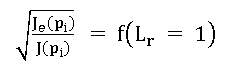
To do so, for each load increment, pi, in a finite element analysis of the flawed structure, the elastic J-integral, J_e(p_i) and elastic-plastic J-integral, J(p_i), are evaluated. The square root of the ratio is then calculated:

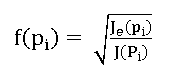
(3)

Depending on the level of the assessment to be performed, the J-based limit load is calculated by finding L_r that satisfies:

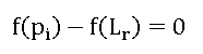
(4)

where

(5)

• L_r is the load ratio, defined as the ratio of reference stress to yield stress, σ_ref/σ_y, or applied load to limit load, p_i/p_L.
• E is the Young’s modulus.

and

• ε_ref is the reference strain corresponding to σ_ref from the stress-strain curve of the material.

This allows for the limit load (reference stress) to be determined for every load increment, and consequently L_r can be plotted against any loading parameter such as remote applied stress and strain.

2.6 Approach of Zerbst et al

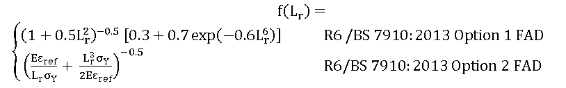
The approach of Zerbst et al ^[6] for evaluating J-based limit loads is essentially equivalent to the API-579 method, except that it is posed in terms of the Option 2 R6 FAD. Define the R6 Option 2 FAD by:

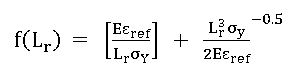
(6)

Then, when the applied load p is equal to the reference load p_L, then L_r = 1, the reference stress is identical to the yield strength and εref is the corresponding strain. The value of f(L_r = 1) is obtained from Equation ^[5] and this in turn corresponds to:

(7)

3. Canadian pipe bend (CPB) tests

3.1 Experimental data

Large- and full-scale tests offer a powerful route to validating ECA procedures, as described in Chapter V of R6 and in background documents to BS 7910, eg Hadley and Moore, 2006 [7]. Whilst it is relatively easy to introduce artificial through-thickness and surface‑breaking flaws into test specimens, there are very few published tests featuring embedded (buried) flaws. Exceptions are the work on flat plates carried out by Willoughby and Davey (referred to in the companion paper), and a set of two tests on pipelines, reported by Coote et al (1985 ^{[8] [8a]}) as part of a much larger series of tests carried out on behalf of the CSA (Canadian Standards Association) in support of the standard Z184 for gas pipeline systems.

Of particular interest amongst the pipes tested for the CSA are two containing circumferential embedded defects in the girth weld, and only these (specimen nos. 16 and 17 in the original work) are considered further in this paper, since they represent some of the very few full‑scale tests carried out on pipes containing embedded flaws.

The welds were in the as-welded condition and loaded in bending. The pipe and flaw dimensions are shown in TABLE 1. The characteristics of the pipe (large diameter/thickness ratio) and the flaw (high length/through-wall height ratio) meant that it lay outside the range of the models and parametric equations developed by Cheaitani and Goldthorpe, so the approach described in the companion paper could not be applied (the equivalent flaw size parameter, α’’, was 0.37 for these tests, compared with α’’≤0.25 for Cheaitani and Goldthorpe’s work).

TABLE 1 - Pipe and flaw dimensions of the Canadian Pipe Bend tests with embedded flaws. Reproduced from Challenger et al (1995 ^[9])

Specimen No.	Pipe diameter, mm	Wall thickness, B, mm	Flaw length, 2c, mm	Flaw height, 2a, mm	Ligament height, p, mm
16	914	10.28	300	4.1	1.5
17	914	10.28	300	3.6	1.5

 

TABLE 2 - Canadian pipe bend tests – materials properties. Reproduced from Challenger et al [9]; Kmat calculated in accordance with BS 7910:2013 ^[2]

Specimen Nos. (Challenger et al)	Tensile Properties		δmat, mm	Kmat, MPaÖm
	σy, MPa	σF, MPa
16 & 17	689	758	0.1	159

 

For the tensile properties, yield strength and flow strength (but not UTS) are cited, with the values for Specimens 16 and 17 shown in TABLE 2. Tensile properties suggest a grade of API X100. Fracture toughness was determined in terms of CTOD (d), with characteristic value δ_mat=0.1mm. In order to allow presentation of the results in terms of L_r and K_r as per R6/BS 7910 conventions, this can be converted to a value of K_mat=159MPa√m. The test was stopped when buckling intervened.

The CPB tests have previously been assessed in terms of earlier editions of BS 7910 ^[7] and its predecessor, PD 6493 ^[9]. The values of Lr attained (calculated using the BS 7910 approach) were 2.03 (for specimen 16) and 1.86 (specimen 17).

Although some data associated with the test are missing, these two tests represent some of the very few full-scale tests carried out on embedded flaws. Attempts were therefore made to model one of the tests as described below.

3.2 Numerical modelling

3.2.1 Method

Bend test no. 16 was re-analysed specifically for this project using FE modelling, with a view to comparing the parametric solutions in R6 and BS 7910 with FEA solutions and actual structural behaviour.

All models were generated using version 6.12-1 of the pre-processing finite element software Abaqus/CAE and the analyses were solved using version 6.12‑1 of Abaqus/Standard (SIMULIA, 2012 ^[10]).

The geometry of the finite element model consisted of a pipe with outer diameter 914mm and wall thickness 10.28mm. The total pipe length was assumed to be 4 outer diameters, ie 3656mm.

For the specific example under consideration, the embedded flaw from CBP Specimen 16 was modelled. This flaw has a total crack height, 2a = 4.1mm, crack length, 2c = 300mm and ligament, p = 1.5mm.

Due to the small aspect ratio (a/c) of the assumed embedded flaw, a canoe‑shaped crack front was employed in the finite element model. This crack front geometry consists of two constant radius arcs (one for the crack front closer to the outer surface and one for the crack front nearer the inner surface) joined at their ends by a semi-circle.

A Cartesian coordinate system was employed with the x-axis along the axis of the pipe. Due to symmetry considerations with respect to the geometry and the applied loads, one-quarter of the pipe was modelled, with an axial symmetry plane along the crack plane, and a longitudinal symmetry plane. Figure 1 illustrates the quarter pipe geometry and crack position.

All models were meshed with 20-node, quadratic, hexahedral, reduced integration elements (type C3D20R in Abaqus). The region near the flaw was meshed densely and smoothly transition to a coarser mesh away from the flaw. The traditional swept, spider web crack tip mesh was employed, with rings of elements structured around the crack front and a tube of degenerate wedge elements enclosed the crack tip.  For the linear elastic simulations, the mid-side nodes of the wedge elements were shifted to the quarter-point position in order to accurate resolve the linear elastic 1/√r singularity, and single-node degeneracy was employed. For the elastic-plastic simulations, the mid-side nodes of the wedge elements were left un-shifted, and duplicate node degeneracy was employed at the crack tip. Several images of the finite element mesh are shown in Figure 2.

The ultimate tensile strength, σ_U, was estimated as 827MPa from the yield and flow strength. In order to allow for some strain-hardening behaviour in the elastic-plastic FEA (for the J‑based limit load calculation) the yield strength and ultimate tensile strength were used to construct a bilinear stress-strain curve. A conservative value of 5% (total engineering strain) was assumed. The stress-strain curve was converted into true stress and true plastic strain for input into the finite element model. A rate-independent plasticity model using the von Mises yield criterion and isotropic strain hardening rule was adopted for the finite element models.

In the finite element simulations, the following material properties were used:

• To calculate the stress intensity factors, only linear elastic properties were used.
• To calculate the limit load based on the spreading plastic zone method, an elastic-perfectly-plastic material model was used.
• To calculate the limit load using a J-based method, the bilinear stress-strain curve converted to true stress-strain was used.

In order to apply a remote axial force or global bending moment to the pipe model, a reference node was created along the pipe axis at the end of the pipe in the positive x-axis, and the free end of the pipe was kinematically coupled to the reference node (see Figure 2). Three sets of applied loads were considered for the linear elastic analyses:

• Axial stress. A uniform 1MPa axial stress was applied to the model by applying a concentrated force at the reference node.
• Global bending stress. A 1MPa global bending stress was applied to the model by applying a concentrated moment about the z-axis at the reference node.
• Simulated residual stress (crack flank pressure). A 1MPa pressure was applied to the crack flank on the symmetry plane in order to simulate uniform, tensile residual stresses acting on the flaw section.

For the limit load simulations with elastic-plastic material properties, a concentrated moment was applied to the reference node to achieve a target (elastically-calculated) global bending stress of 690MPa. This value was chosen as it is the reported failure stress of Specimen 16 from the CPB trials.

Due to the assumed quarter symmetry, two symmetry plane boundary conditions were assigned. All faces along the longitudinal symmetry plane were restrained in the z-direction (U3=0) and all faces along the axial symmetry plane were restrained in the axial direction (U1=0). Figure 2 illustrates the loads and boundary conditions.

3.3 Results

3.3.1 Stress intensity factors

For each of the linear elastic simulations, History Output Requests were created in Abaqus/CAE to evaluate the stress intensity factors (K_I, K_II, and K_III) and the J-integral from 10 contours surrounding the crack tip. Each simulation was checked to ensure that the output values of stress intensity factors and J-integral had converged by the outermost contour; that is, path-independence of the J-integral was obtained. Therefore, in what follows, the values reported for a given crack are the path-independent, converged values from the outermost contour.

Three linear elastic loading conditions were considered: axial stress, global bending stress and crack flank pressure. For each set of applied loads, the stress intensity factors were evaluated at each node along the crack front. The crack front was parameterised in the usual manner by the parametric crack front angle, ranging from 0° at the point of the flaw along the longitudinal symmetry plane, closer to the outer surface of the pipe, to 180° at the point of the flaw along the longitudinal symmetry plane, closer to the inner surface of the pipe. In Figure 3 the mode-I stress intensity factors (K_I) is plotted against the parametric crack front angle. It can be seen that, due to the large ratio of outer diameter to wall thickness, there is very little difference between the results due to global bending stress and axial stress (ie there is very little through wall bending).

The maximum values of K_I along the embedded crack front for each loading condition are as follows:

• 1MPa axial stress: 3.149MPa√mm.
• 1MPa global bending stress: 3.131MPa√mm.
• 1MPa crack flank pressure: 3.130MPa√mm.

For the fracture assessment, a global bending stress of 690MPa was assumed and the residual stresses were assumed to be yield magnitude. Therefore:

• KI^P = 2160MPa√mm (68.3MPa√m).
• KI^S = 2160MPa√mm (68.3MPa√m).

3.4 Limit load based on spreading plastic zone

For the elastic-perfectly-plastic analysis, the applied moment was increased incrementally until the plastic zone spread through the smallest ligament. The moment was applied so that at a load amplitude of 1.0, the pipe would experience an elastically-calculated global bending stress of 690MPa. Plastic collapse occurred at load increment 0.4938, hence the collapse stress was 0.4938 x 690MPa = 340.72MPa. By taking the ratio of applied stress to collapse stress, L_r can be calculated as 690MPa/340.72MPa = 2.02. The plastic zone at collapse is shown in Figure 4. As previously discussed, this case represents a geometry where one ligament is significantly smaller than the other (ie 1.5mm versus 4.68mm). Consequently, if the collapse stress is calculated from the moment required to cause the plastic zone to snap through the larger of the two ligaments, then L_r is less than 1.75. A comparison of existing embedded flaw reference stress solutions with the two different formulations of the spreading plastic zone method is the subject of on-going research.

3.5 Limit load from J-based method

In Figure 5 the elastic and elastic-plastic J-integrals are plotted against the applied global bending stress. By evaluating the BS 7910:2013 Option 1 FAD and the BS 7910:2013 Option 2 FAD at L_r= 1:

f₁ (L_r=1)=0.673 [7]

f₂ (L_r=1)=0.816 [8]

is obtained.

Note that two different stress-strain curves were employed for the Option 2 FAL: the bilinear stress-strain curve and a Ramberg-Osgood fit (as described in BS 7910:2013 Clause 7.1.3.5) through the yield and ultimate tensile strengths used to define the bilinear curve. However, for this case, the choice of stress-strain curve (discontinuous vs continuous yielding) does not affect the value of the failure assessment line at L_r= 1.

According to the J-based limit load method, in order to determine the reference stress, the global bending stress for which √(J_e/J) equals either value in Equation [7] needs to be solved for. This is illustrated graphically in Figure 6.

Therefore, the reference stress is 403MPa for the Option 1 assessment and 365MPa for the Option 2 assessment. The corresponding load ratios, L_r, can be evaluated by dividing the reference stress by the yield stress, giving L_r = 1.71 for the Option 1 assessment and L_r = 1.88 for the Option 2 assessment.

4. Discussion

As seen in Figure 7, the results of three different FEA-based analyses (spreading plasticity method, plus methods based on the Option 1 and Option 2 FADs) produce lower values of the plasticity parameter L_r than the values derived from BS 7910 or from the local collapse formulations in R6. Note that the FADs (including the Option 3 FEA-based FAD) have been truncated at a value L_r,max=σF/σY =758/689=1.1 in Figure 7, in accordance with the conventions of R6 ^[1] and BS 7910 ^[2], although the Option 3 FAD could have been extended to higher values of L_r to show more clearly the relationship between the FAL and the data points associated with the FEA.

Recently (subsequent to the publication of the FEA carried out by Cheaitani and Goldthorpe), TWI has developed a software tool for the rapid generation of FEA meshes in pipes and other components, which has the potential to bypass some of the issues encountered by Cheaitani and Goldthorpe. The methods discussed in this paper are being further developed and applied to a range of geometries, with a view to validating and verifying the conclusions of the work carried out to date.

5. Summary, Conclusions and Recommendations

1. Experimental validation of limit load/reference stress solutions for embedded flaws in both flat plates and pipes is very limited: just two sources of data have been traced and re-examined in this work. These constituted a series of flat plate specimens containing artificial embedded flaws (discussed in the companion paper) and a pair of pipe bend tests carried out in support of the Canadian Standards Authority ^[8].
2. An alternative approach to the calculation of limit load/reference stress is to use Finite Element (FE) Analysis, adopting either a spreading plastic zone method or a J-based method. The latter requires direct elastic-plastic FE modelling of a flawed component, then forcing a fit between the Option 3 FAD produced by FEA and the Option 1/Option 2 FAD as defined in R6 and BS 7910.
3. By employing J-based limit load calculations for the re-analysis of the embedded flaw in a specimen from the Canadian Pipe Bend trials, some of the conservatism arising from the use of flat plate solutions in R6 and BS 7910 can be removed. This is seen by a shift in the L_r values to the left, closer towards the failure assessment line (but still remaining outside it).

6. Acknowledgements

This publication is based on work carried out by TWI on behalf of the R6 panel, described in full in Hadley and London (2015 ^[11])

7. References

1. BEGL, Assessment of the integrity of structures containing defects, R6 Revision 4 and amendments, British Energy Generation Ltd, Gloucester, UK (Amendment issued in subsequent years), 2001
2. BSI, Guide to methods for assessing the acceptability of flaws in metallic structures, BS 7910:2013, British Standards Institution, 2013.
3. Hadley I, Tyler L and Cheaitani MJ, Analysis of limit load for embedded flaws in pipeline girth welds, Part I: Review and validation of current procedures, this conference, 2015
4. API, Fitness-for-service, API 579, First Edition, American Petroleum Institute, 2000
5. API/ASME, Fitness for service, API-579-1/ASME-FFS-1-2007, API 579 Second Edition, American Petroleum Institute (API)/American Society of Mechanical Engineers (ASME), 2007
6. Zerbst U, Ainsworth R A and Madia M, Reference load versus limit load in engineering flaw assessment: A proposal for a hybrid analysis option, Engineering Fracture Mechanics 91, 62-72, 2012.
7. Hadley I and Moore P, Fracture case studies for validation of fitness-for-service procedures, TWI Member Report 850/2006, Abington Hall, United Kingdom, 2006
8. Coote R I, Glover A G, Pick R J, Burns D J, Alternative girth weld acceptance standards in the Canadian gas pipeline code, Paper 21, Proceedings of the 3rd International Conference on Welding and Performance of Pipelines, 18-21 Nov 1986, London, UK, pub The Welding Institute, 1987, ISBN -0-853-00213-4, 0-853-00215-0, 1985
9. (8a)   Coote RI, Background to alternative standards of acceptability proposed for CSA Z184, Girth Weld Defect Task Force, CSA Joint subcommittee on joining, March 1985.
10. Challenger N V, Phaal R and Garwood S J, Appraisal of PD 6493:1991 Fracture assessment procedures Part II: Published and additional TWI data, TWI Member Report 512/1995, Abington Hall, United Kingdom, 1995
11. SIMULIA, ABAQUS/Standard User’s Manuals, Simulia, 2012.
12. Hadley I and London T, Assessment of limit loads in circumferential embedded flaws in pipes, TWI report 23887/2.1/15, January 2015

 

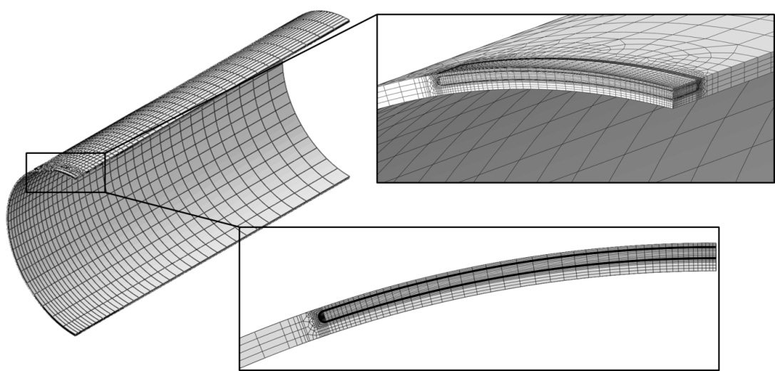
Figure 1 Geometry and finite element mesh for Specimen 16.

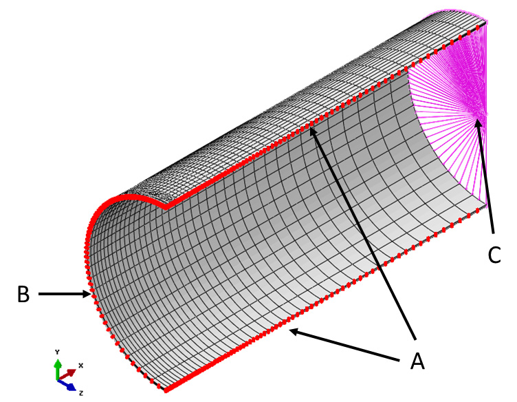
Figure 2 Loads and boundary conditions for the embedded pipe model. A – Z symmetry B – X symmetry C – Loading sleeve

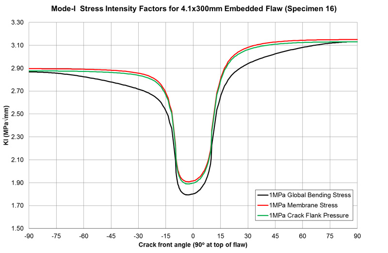
Figure 3 Stress intensity factors along the embedded crack front under unit global bending stress, axial (membrane) stress and crack flank pressure.

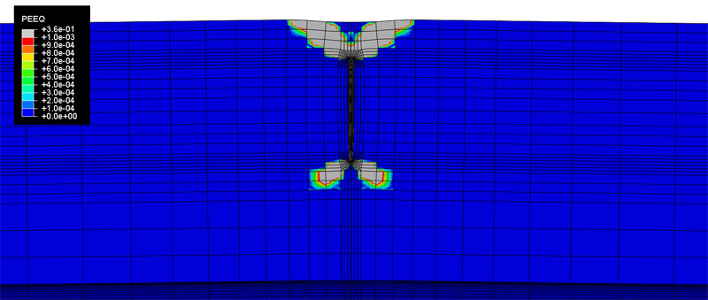
Figure 4 Equivalent plastic strain (PEEQ) contour on the pipe along the longitudinal symmetry plane at plastic collapse as determined by the spreading plasticity method. Deformation magnified by a factor of 10.

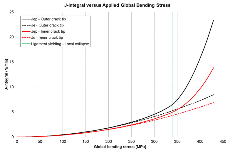
Figure 5 Elastic and elastic-plastic J-integral at the position of the flaw experiencing the largest crack driving force.

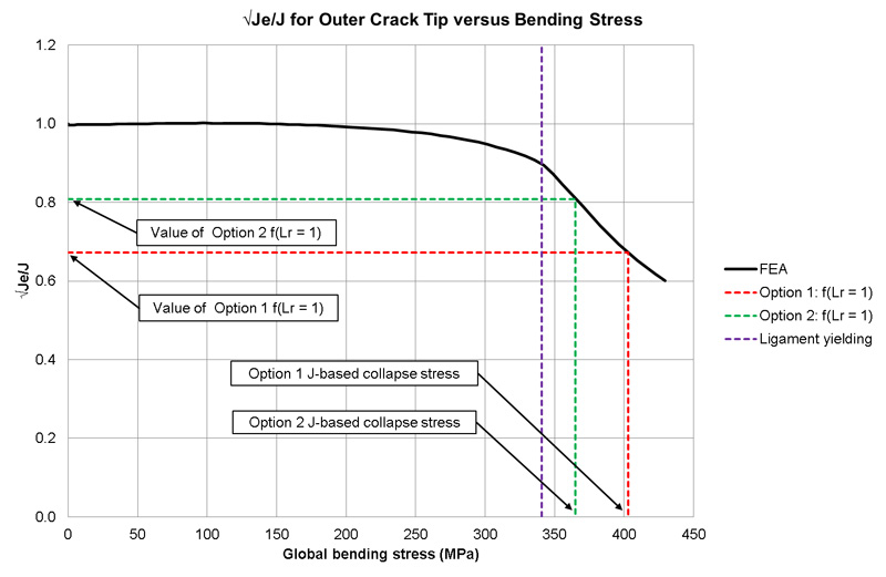
Figure 6 A plot illustrating the evaluation of the reference global bending stress for the J-based limit load calculation.

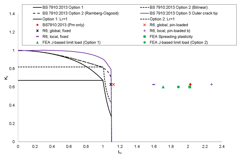
Figure 7 Failure assessment diagram for different assessments of the same flaw.